Kater Pendulum Theoretical Considerations
Randall D. Peters
Department of Physics
Mercer University
Macon, Georgia 31207
1 Idealized Kater Pendulum
Consider a uniform
rectangular pendulum as illustrated in Figure 1. One axis of rotation is
an end, and we wish to find another axis for which the periods of oscillation
about the two parallel axes are the same. Note that the pendulum must be
turned upside down to oscillate about axis 2, the adjustable knife edge.
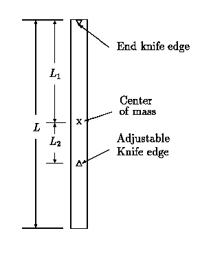
Figure 1: Illustration of a simple Kater pendulum.
For small amplitudes of free decay,
the equations of motion are given by Ii d2q/dt2 + MgLiq = 0;
and the moments of inertia are
by use of the parallel axis theorem.
If the pendulum length L is considerably greater than its width or
thickness, then the center of mass moment is given by
Ic = ML2/12.
Additionally, L1 = L/2, and L2 is to be determined.
From the solution
to the equation of motion, the periods are found to be
It is convenient to define the radius of gyration, k, whereby
Ic = Mk2. From equations 1 and 2, the condition T1 = T2
requires that
|
k2 = L1L2 for period matching |
| (3) |
Additionally, since k = L/121/2, we see that
L2 = k2/L1 = L/6.
Thus, for the matched condition,
|
T1 = T2 = T = 2p[(L1 + L2)/g]1/2 = 2p[2L/(3g)]1/2 |
| (4) |
We thus see that the pendulum, for the matched period condition, is
equivalent to a simple pendulum of length 2L/3.
1.1 Variation of Period with Axis Position
It is
instructive to consider the pendulum as outfitted with a hypothetical
single axis, rather
than the two required for operation, and look at the variation of period
with the position y of this
single axis relative to the center (of mass) of the pendulum, in the range
from 0 < y < L/2, as shown in Figure 2.
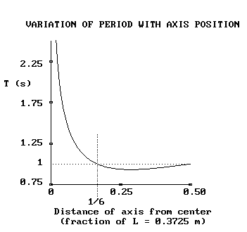
Figure 2: Period vs axis position for a pendulum of Figure 1 type.
The first thing one should note from Figure 2 is that there are two cardinal
axis positions-one at L/2 and the one which yields the same period
at L/6. The length of the pendulum for Figure 2 was chosen at
L = 37.25 cm to yield a 1 s period when g = 9.803 m/s2.
2 Non-Ideal Features
2.1 Effect of Period Difference
Ultimately, there will always be a measurable difference
between the periods, T1 and T2, but attempts
to match them is an exercise that is unnecesary, since the effect of
small difference can be factored
into one's estimate for the acceleration of gravity g .
Imagine that the position of pivot 2
could be changed by a small amount, D, from
its nominal L/6 from the center of the pendulum.
(In our initial consideration of the influence of departures from ideal
geometry, the offset distance of pivot 1 from the end of
the pendulum will be ignored-a complication which will be addressed later.)
The dependence of T2 on D is determined by two factors: (i) the
moment arm of the gravitational force and (ii) the change in the moment of
inertia about the pivot (readily calculated using the parallel axis theorem).
The period is found to obey
which is seen to equal T1 when D = 0.
Assume that one makes an accurate measurement of the separation distance
between the two pivots
By expanding the square root term in (5) with the binomial theorem
and retaining terms only to
first order in D, one obtains
which combines with (6) to yield
The usefulness of (8) derives from the manner in which lm changes with
the ratio T2/T1.
If T2/T1 > 1 then lm < 2/3L. On the other hand if
T2/T1 < 1 then lm > 2/3L. Moreover,
Equation (8) provides automatic compensation over a surprisingly large
range of deviations in DT = T2-T1, for reasons that can be
appreciated qualitatively
by studying Figure 2.
A quantitative indicator of the compensation of Eq. 8 is
provided in Figure 3.
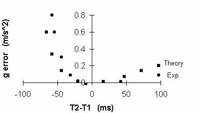
Figure 3: Errors of Eq. 8
To generate the experimental results, a very crude
pendulum was cut out of aluminum with a hacksaw to the approximate size of
the TEL-Atomic instrument. An end 1/4 in hole was drilled for axis-1, and
7 axis-2 holes were drilled at various positions around the 2L/3 point. The
total range of distances between the axes was 5.7 cm. In this range, the
period difference
T2-T1 varied from -58 ms at 28.2 cm separation to 97 ms at 22.5 cm
separation of the axes.
Eq. 8 is not capable of fully describing this
system because it corresponds to a 2-hole pendulum rather than the 7-hole
pendulum tested. Nevertheless the equation fits the data reasonably well
as shown in Figure 3. Interestingly, over the full 5.7 cm range, the largest
error in the g estimate does not exceed 8%. Moreover, for a certain 3 cm
range (favoring smaller as opposed to larger than nominal separations), the
error does not exceed 1%. For tolerances on hole placement held to
approximately 1 mm, Eq. 8 results in errors not to exceed 1 part per 10,000.
It is worth repeating-errors in the placement
of the axis-2 hole are less significant if its placement is shy of
(as opposed to greater than) the
L/6 nominal distance from the center.
One must recognize a shortcoming to the utility of Eq. 8 as compared to the
more elaborate method of using a small mass slider as described in
the operational part of this manual. The relative uncertainty in the
estimate of g, when using eq. 8 is given by
|
dg/g = [(dlm/lm)2 + (2dT2/T2)2 + (3dT1/T1)2)]1/2 |
| (9) |
Weighting by the factor of 3 in the T1 errors (due to the cubic term)
requires more careful period measurement as compared to
the slider method.
In spite of the extra contribution to the uncertainty in g, Eq. 8 is
still quite useful. For example, it was used with the data obtained
from the TEL-Atomic pendulum employing a 2.6 g slider. The errors of
Fig. 4 derive from the calculation of g by means of quadratic
fits to the T1 and T2 data. They are seen to be less than one
part per thousand for every position of the slider between 0 and 30 cm.
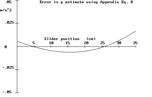
Figure 4: Errors in g estimate using Eq. 8 on TEL-Atomic pend. with slider
3 Practical pendulum
The idealized rectangular pendulum treated above is not practical, since
axis engineering has been ignored. Some things that were
tried unsuccessfully involved (i) bearings mounted in the pendulum for
sharpened pins to ride against, and (ii) small cylinders inserted
through the
pendulum. The only practical means found for providing axes
is the scheme next described, involving a pair of holes drilled through
the pendulum.
3.1 Configuration with a pair of holes for a knife edge
Let each hole be of radius r, their centers being located
at y1 (positive) above the center of the pendulum, and
y2 (negative) below the center. Since y2 is in magnitude less than
y1, there is a small negative shift of the center of mass of the pendulum
with respect to the center of the rectangle (-0.8 mm for the TEL-Atomic design).
The position of
the center of mass is given by
|
yc = -p r2(y1 + y2)/(Lw - 2pr2) |
| (10) |
where L is the overall length of the pendulum and w is its
width.
If there were no holes in the pendulum, its mass normalized
moment of inertia, with respect to the center of mass
(c.m. = geometric center), would be
|
Ic, ideal = (L2 + w2 )/12 |
| (11) |
where t is the thickness.
Although the term involving t = 0.32 cm is presently ignorable, the one
involving w = 1.3 cm
is not (as compared to L = 37.4 cm). To match the periods about the two axes to a few parts in 10,000
requires the computer. The easiest way to accommodate the holes
is to treat them as negative masses. By using this technique and
the parallel axis theorem, one obtains
the following expression for the nonideal mass normalized c.m. moment:
|
Ic = [(L2+w2)Lw/12+Lwyc2-pr2[(y1-yc)2+(y2-yc)2]-pr4]/(Lw - 2pr2) |
| (12) |
To estimate the period for each of the axes, it is necessary to
specify the distance of each axis from the center of mass:
d1 = y1 + r - yc
d2 = y2 - r - yc |
| (13) |
in which care must be taken with regard to algebraic signs.
Using then the moments of inertia
I1 = Ic + d12
I2 = Ic + d22 |
| (14) |
the periods are found to be
T1 = 2p[I1/(gd1)]1/2
T2 = 2p[I2/(g(-d2))]1/2 |
| (15) |
3.2 Design of the TEL-Atomic pendulum
The holes were selected to be 0.25 in diameter, and w = 1.3 cm so
that the amount of side material at the axis-2 position would be
adequate for structural integrity. Similar considerations figured
into the placement of the axis-1 hole; i.e., the distance from the center
of the pendulum was chosen at 18.18 cm to give a 2 mm piece of
metal where the knife edge rides.
The length L = 37.4 cm and the axis-2 hole position of y2 = -5.995 cm
were obtained by programming the computer
with the equations given above, and allowing L and y2 to vary.
The objective was to select for these values a matched
condition corresponding to a period of 1 s.
For a small set of L values (expected from idealized pendulum
considerations to be in the neighborhood of 37 1/2 cm), y2 was
allowed to vary quasi-smoothly through a range which permits T1 = T2.
In the calculations, g was set to 9.797, and
the matched period condition is one which yields for the estimated
acceleration of gravity
g = 4p2 (d1 - d2)/T2, T = T1 = T2
with d1 = 18.58 cm, d2 = -6.232 cm |
| (16) |
Note that the nominal simple pendulum equivalent length is
d1 - d2 = lm (Eq.8) = 24.81 cm.
For the indicated parameters, the nominal period values were
T1 = 0.9998 s and T2 = 0.9999 s. Attempts to get
closer to unity
were found to be futile for reasons that probably derive from
the brass of the pendulum being less than perfectly homogeneous in
terms of mass density.
For example, one pendulum to the next typically shows deviations from the
nominal periods on the order of 5 parts per 10,000.
File translated from TEX by TTH, version 1.95.
On 19 Nov 1999, 11:23.