Tutorial on Power Spectral Density Calculations
Tutorial on Power Spectral Density Calculations for Mechanical Oscillators
( with an exhaustive discussion of Units )
Randall D. Peters
Physics Department, Mercer University
Macon, Georgia
Copyright January 2012
Abstract
This article provides a thorough description for the calculation of power spectral densities (psd) based in simulations of a classical harmonic oscillator with damping due to an external viscous force. Self consistency of information between the domains of time and frequency results in a single natural set of units for the psd. For a graph generated with an axis that is linear in frequency, this set of psd units is w/kg/Hz, which is equivalent to m2/s3/Hz. For a logarithmic frequency scale, the natural units are watts per kilogram per one-seventh-decade. A simple transformation yields the psd from the commonly employed acceleration spectral density (asd) whose units are m2/s4/Hz (or g2/Hz). Only after doing this transformation does one obtain a density function that has meaning in a true-power
sense. This is especially important for calculating a quantity like total seismic background noise power.
Introduction
Starting about 1900, some of the most important advances in physics were made possible through spectral analysis. These
were central to the development of the quantum mechanics that has greatly impacted the modern world, including even the computer with which this article was written. A classic example relevant to present considerations was Einstein's derivation of the Planck distribution of black-body radiation. The thermal power generated by a body because of its temperature can be specified either in terms of frequency (n) or wavelength (l). Their inverse proportionality (l Á 1/n) through the speed of light c, has profound influence because the specification of the radiated power density necessarily includes a differential that is one or the other of dn or dl. The relationship dl = -dn / n2 is responsible for two different functional forms for the power density spectrum, depending on whether it is expressed in terms of l or in terms of n.
In similar manner, there is a very important difference between a mechanical system density graph specified in terms of (i) frequency f as opposed to its close-neighbor graph in terms of (ii) Log(f). This difference derives from the fact that a differential is associated with every density function. The differential df for (i) is not rigorously suitable for (ii), because the latter is most properly d[Log (f)]. Because d[Log (f)] Á df / f, an additional s-1 (corresponding to the unit Hz of f, in honor of Heinrich Hertz) is inextricably involved in every tranformation between the two distributions. Huge errors can be generated if this difference is not recognized and correction made for it, as illustrated in Fig. 1.
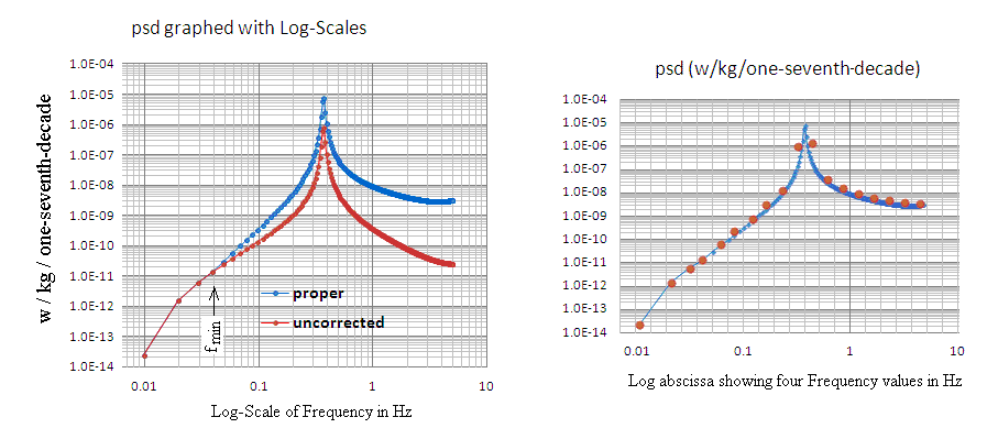
Figure 1. Demonstration (left) of the need to correct the psd when going from a Linear-Frequency scale to a Log-Frequency scale.
The right graph provides values (red dot centers) for the power in a given logarithmic bin, each of which has a width of one-seventh of a decade. The theoretical basis for these graphs is provided in discussions of the `model system' that follows.
The uncorrected continuous red curve was obtained from a proper psd by simply replacing its Linear-Frequency scale with a Log-Frequency
scale. Although frequencies can be readily read from the abscissa of this left plot of Fig. 1, the psd units of the proper blue curve are necessarily w/kg/one-seventh-decade and not w/kg/Hz. As is commonly done, one can work with the red curve of the left plot and declare
its units to be W/kg/Hz. To do so requires `mental gymnastics' in which an association is made with the linear graph from which the log graph was derived. Doing so has caused great confusion, and the need for better widespread understanding of power spectral density is paramount. Only then can total power in watts be calculated without unreasonable errors. Accurate total power calculations
using frequency domain data would greatly improve our understanding of the physics for a host of important systems.
Consider an example of the subtleties that are part of the matter. A popular statement concerning `white' noise is that it is `flat' per Hz. But it is not flat per octave (or decade or fraction of either); rather it shows a dependence on f to the first (positive) power. On the other hand, `pink' noise which shows 1/f dependence in
a log-log plot of per Hz type becomes `flat per octave'. In one of the simulations that follow, the drive involves 1024 random
number variates governed by a normal distribution. For this case the drive acceleration is in the form of `white' noise. For all of
the several simulation cases considered, it will be shown that the true (specific) power spectral density results from one cause only. It is the work done per unit mass by the external force, against the damping force of the oscillator. This work is simply the product of the damping force and the velocity. Because the velocity at steady state is proportional to acceleration divided by frequency, we conclude that the power spectral density plot will be flat per octave. It is therefore an example of `pink noise'.
The correction shown in the left plot of Fig. 1 is performed by multiplying every psd component of the spectral set by its associated (unique) frequency f, and then dividing the resulting product by a minimum frequency fmin, The lowest frequency component above zero = d.c. of the spectrum is given by f lowest = ( fs / 2 )( 1 - 2 / N) / ( N / 2 - 1 ), where fs is the sample rate (reciprocal of the delta time between samples). The total number of spectral points (both positive and negative frequency components) is N, and the Nyquist (highest) frequency is given by f Nyquist = ( fs / 2 )( 1 - 2 / N). Only positive frequency
components are considered, and so the values for the square of the modulus of the FFT used in calculating the psd are each multiplied by a factor of two.
Starting at f Nyquist (4.99 Hz in the figure) and moving downward, fmin corresponds to the frequency of the first-encountered one-seventh-decade bin that contains only a single point. As the frequency increases above fmin, the number of points per bin increases. There is a single spectral point in the bin containing 0.04 Hz. For the bin containing 0.3 Hz there are 11 points, and their sum yields the value (approx. 1 E-06) corresponding to the red dot just to the left of the peak
corresponding to the oscillator's natural frequency.
If the bins were all one octave in width, every doubling of the frequency would result in a doubling of the number of points per bin.
Keep in mind that no abscissa involving a math function can legitimately contain any unit(s), and that d[Log(f)] is acceptable since it is dimensionless. Consequently, the only differential that makes rigorous (formal) sense when graphing a density function involving the logarithm is either (i) octave, or (ii) decade, or a specified fraction of either. A useful choice, for ease of making the red dots of
Fig.(2) fall close to the curve indicated is one-seventh of a decade. The bins in the right plot of the figure were generated using
Log[f]/Log[10(1/n)], where n = 7 and the Log is base 10. The value of n = 7 is a convenient choice, in that smaller n yields a sparsely populated graph. Increasing n causes the shape of the graph to be increasingly distorted at low frequency, depending on the size of N, the
number of FFT points. This distortion derives from the presence of unpopulated bins, and an example of such is visible from the figure (the
bin adjacent to the one containing the lowest frequency). For common values of N = 1024 or 2048, n = 7 is a good choice.
An example from common practice also illustrates the great need for care when working with log plots. It involves the
change that occurs when a spectrum is plotted versus period rather than the equivalent spectrum plotted versus frequency. It is well known that when the abscissas are both log scale, that the two graphs are simply mirror images of each other, as shown in the top pair
of plots in Fig. 2.
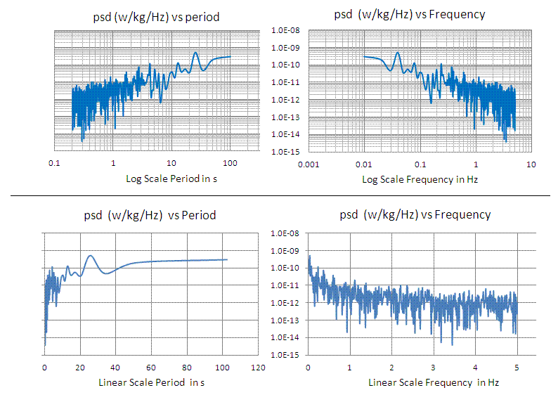
Figure 2. Pink noise spectra illustrating differences between psd versus frequency and psd versus period. The model system
case that was simulated to produce these graphs is discussed later in detail.
The reason for the top pair of graphs in Fig. 2 being mirror images of each other is easy to understand. It results because d[log(T)] = dT/T = - df/f = - d[log(f)].
In other words, their differentials, neither of which has any units, have the same magnitude. When expressed in terms of
w/kg/(decade/7) the total power is obtained simply in the same way from either of the two graphs, by summing up all the ordinate
values, for which there is a single number for every seventh-decade bin.
On the other hand, the lower pair of graphs of Fig. 2 dramatically illustrates the profound difference that results when the density functions
are expressed in linear abscissa form. The power estimated by means of ‗ psd(f)df is not the same as the one
involving ‗ psd(T)dT, where frequency is simply converted to period, as was done in the log plots. The difficulty derives from the requirement that
|psd(f)df| = |psdó(T)dT|, where the primed distribution is obtained from the unprimed one by dividing every component in the frequency set by T2. Let f « x so that the specific power in watts is given by P/m = ‗ psd(x)dx. If one does the
same integral in terms of T « y, then the same results are obtained when the integral used is -‗ (1/y2)psd(y)dy.
This was demonstrated to be true for the simulated pink noise example. It is important when doing the integral over period to recognize that the (negative) delta T employed is not constant, as is true of df for the frequency based integral. The right-side plot of Fig. 3 shows how the magnitude of delta T decreases as frequency increases, and the left-side plot was obtained from the lower left graph of Fig. 2
by dividing its values by T2.
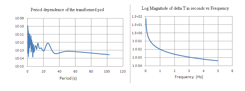
Figure 3. Illustration of the transformation of psd that is required when working with period rather than frequency, and also using a linear abscissa.
Parseval's Theorem
In the analyses that follow, it is important that we recognize a quintessential equality. The theorem given us by Parseval involves a requirement that is placed on power. It forces a precise relationship between a time dependent signal and its associated Fourier transform calculation. Only one `normalization' of the frequency domain data obtained with the transform is acceptable; i.e., the one for which the rate with which energy is transferred must be the same, whether calculated in the time domain or the frequency domain. Anything else is in violation of the requirement that total energy be conserved; it can be neither created nor destroyed, rather only change in form.
Parseval's theorem was obeyed by the algorithms used in the generation of Fig.(1), as will be demonstrated. Consider first the sum of the ordinate values for the eighteen (equally-weighted-at unity) red dots in the right plot of Fig. 1. From the Excel spreadsheet used to generate the figure, their sum was found to be 2.47 × 10⁻⁶ w/kg. The same total (specific) power was also calculated by summing over the 512 values responsible for the red curve of the left plot of Fig.(1). It will be shown in the theoretical section to follow that this
corresponds to the amount of power per kg expended in the form of heat as a 2-kg mass oscillates with a frequency of 0.356 Hz in exponential free-decay, starting from rest with a displacement of 1 cm.
Important Note
It should be pointed out that none of the various FFT algorithms known to this author actually calculates the spectrum in terms of
`Hz'. Instead, the spectral density that is generated contains a total number of N/2 equally spaced `points' that are separated from one
another by approximately df = fNyquist/(N/2). To properly calculate the total power using ‗ P(f)df (should one choose to do so), it is necessary to divide each of the spectral values in W/kg/FFT pt. by df. It is more convenient to avoid this complication and simply sum over all the points.
We see then that it would be more precise to label the majority of spectra with `per FFT point' rather than with `per Hz'.
Yet another subtlety of most FFT algorithms needs to be recognized, if one is to properly estimate absolute powers. To minimize memory
requirements of the algorithm, a given array gets filled with numbers that change from one filling of the array to the next required filling to complete the calculation. Proper normalization of the
final result requires that the output be corrected by a scale-factor. In the case of the Excel algorithm, every real and imaginary
component of the output must be divided by N, the total number of components used in the calculation of the FFT. Thus, for every
calculation of this article, the modulus values for a given spectrum were devided by 10242 = 1.049 × 10⁶. On the other hand,
if these calculations had been done with Mathematica, the appropriate factor would have been 1024 rather than its square.
Model System Components
With attention to the aforementioned issues, we look now at the system that was chosen for the focus of this tutorial. It involves an idealized massless spring that obeys Hooke's law. (That such a spring does not in reality exist is presently irrelevant.) The magnitude of the spring constant k, along with the mass m that is attached to the spring on one end (whose other end is constrained to be stationary with respect to the box holding the oscillator), determines the frequency fo with which the system oscillates. The linear second order homogeneous differential equation that describes this oscillator is one of the most famous of all the equations in physics:
|
m |
..
x
|
+ k x = 0 « |
..
x
|
+ wo2 x = 0 , wo = 2p fo |
| (1) |
where a single dot over x implies time derivative; i.e. v = dx/dt. The double dot of Eq.(1) corresponds to acceleration; i.e.,
a = dv/dt = d2x/dt2.
There is no damping term in Eq (1), and as the mass oscillates the total energy is constant with a periodic variation between potential energy of the spring
(U = k x2/2) and kinetic energy of the mass (K = m v2/2).
With damping included
Only after damping is added to Eq.(1) do we obtain something with which this tutorial makes sense. Just as with the idealized spring,
an idealized damping force is assumed for present purposes. It is an external-to-the-spring force called `viscous' and given by
|
ff = - 2 m b |
.
x
|
= - m |
wo
Q
|
|
.
x
|
|
| (2) |
Real springs introduce internal friction to the problem and the `hysteretic damping' that results is nonlinear [1]. Such complications
are not relevant to present purposes.
When the preceding viscous damping force is added, the following equation results:
|
|
..
x
|
+ |
wo
Q
|
|
.
x
|
+ wo2 x = 0 |
| (3) |
It is convenient to integrate Eq.(3) numerically by working with the following (equivalent pair of) first-order coupled equations; i.e.,
|
|
.
v
|
= - ( |
wo
Q
|
|
.
x
|
+ wo2 x ) , |
.
x
|
= v |
| (4) |
The last point approximation (LPA) integration technique is quite adequate to the present case and is easier to implement than a Runge-Kutta algorithm. Fig. (2) shows one result of using the LPA on Eq.(4), with the integration performed in Microsoft's Excel, using
dt = 0.1 s to update the following equations, in the order shown.
|
vn+1 = vn + an dt , xn+1 = xn + vn+1 dt |
| (5) |
Model System 1 - Free decay with damping less than critical
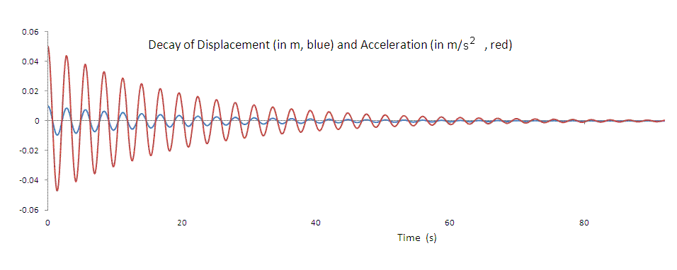
Figure 4. Oscillation with exponential decay of a 2-kg mass affixed to a Hooke's law spring having a constant of k = 10 N/m. The Q of the system is 22.36, determined by b = 0.05 s-1. The mass is released from rest with an initial displacement of 1 cm and
analyzed for 102.3 s; although only about 90 s of the record is shown.
Rate of work done by the friction force
The friction force is seen from Eq.(2) to be proportional to the magnitude of the velocity and opposite to its direction. It causes
mechanical energy to be converted to heat at the following rate per unit mass:
|
|
P
m
|
= 2 b |
.
x
|
2
|
= |
wo
Q
|
|
.
x
|
2
|
|
| (6) |
The dissipated power determined by use of Eq.(6), for the decay of the 2-kg mass shown in Fig. 4, is graphed in the time plot of Fig. 5.
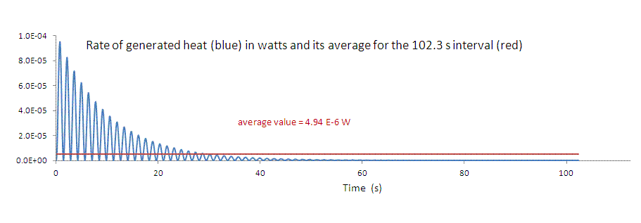
Figure 5. Instantaneous power P (blue) for the conversion of the spring's initial potential energy into heat. The average of
4.94 × 10⁻⁶ w is seen to be identical with the specific power mentioned in the section above, labeled "Parseval's theorem";
since the mass is 2-kg.
Calculation of the Power Spectral Density
It was mentioned earlier that the power calculated using the (specific) power spectral density in w/kg must (because of the mass of 2-kg)
come out to be one half the number 4.94 × 10⁻⁶ w shown in Fig. 5.
That this is the case for the psd used, so that Parseval's theorem is satisfied, will now be shown.
It is simple physics that the instantaneous power (rate at which mechanical energy is converted to heat) is given by the product of the friction force and the velocity. This is the
basis for Eq.(6). For any dynamical system, acceleration is responsible for its motion, so it is here used to calculate the psd. Because
Eq.(6) involves the velocity and not the acceleration, the use of dx/dt = a / wo gives
Observe that the units of psd can only be m2/s3/FFT pt. = w/kg/FFT pt., since the unit of wo is 1/s and Q is dimensionless.
A 1024 point FFT was calculated, using the acceleration values that generated Fig. 4. The square of the resulting modulus values were then used in Eq. (7) to produce the spectra shown in Fig. 6. To obtain the units of W/kg/Hz for the left graph, each value of |FFT(a)|2 was divided by 0.009766 to convert from the w/kg/FFT pt. produced by the Excel discrete Fourier transform algorithm of Cooley Tukey (FFT) type.
The csp was then generated from the psd by a series of discrete numerical integrations; with each of the 512 values using
where the lower limit was flowest = 0.009766 Hz and the upper limit f was stepped progressively from flowest upward to the Nyquist frequency of 4.99 Hz.
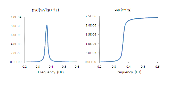
Figure 6. Linear frequency plots of the psd (left) and cumulative spectral power (csp, right). obtained using Eqns.(7) and (8)
respectively. Only a small segment of the total frequency range is shown, centered on the natural frequency of the oscillator.
As expected, these curves show clearly that most of the power is concentrated in a narrow frequency range centered on the natural
frequency of the oscillator. Moreover, the csp is seen to approach (at the Nyquist frequency) the limit of 2.47 × 10⁻⁶ w/kg as required by Parseval's theorem.
Model System 2 - Response to external forcing with near critical damping
Case 1 - a 1 Hz drive acceleration
With near critical damping of Q = 0.5, the oscillator entrains quickly with the drive, which is the modus operandus for a seismometer. Shown in Fig. 7 is the first of several acceleration drives that were chosen for simulation.
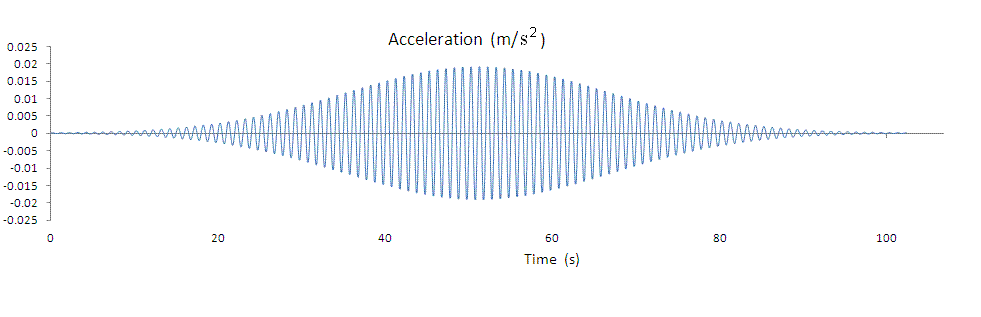
Figure 7. The first drive signal used in simulating the response of the oscillator to an external acceleration. The shape of the envelope was determined by means of a Gaussian.
Previously Q was equal to 22.36 in the decay with damping less
than critical. The damping force, which is independent of
frequency, is determined by b. Its previous value of 0.05 s-1 was changed to b = 1.581 s-1 to yield Q = 0.707, which
is commonly used with seismometers. Note also that the previous frequency term in the psd of Eq.(7) was wo, since it was the only
harmonic acceleration responsible for the generation of heat. For the driven system, wo gets replaced with w (external
harmonic acceleration(s) that does work against the damping force.
So the (specific) Power Spectral Density was calculated using
and used to generate the plots of Fig. 6.
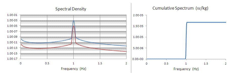
Figure 8. Spectra corresponding to the drive acceleration of Fig. 7. The significant difference, mentioned previously, that is always present between w/kg/(FFT point) (red) and
w/kg/Hz (blue) is illustrated in the left graph.
The cumulative spectrum (right graph) is useful for estimating the total power, which for Fig. 8 was 1.67 × 10⁻⁵ w/kg. Using Eq.(6) this was found (within errors of numerical integration) to be the same as the total power dissipated by work against the damping force of the oscillator.
Case 2 - a 3 Hz drive acceleration
To demonstrate the validity of Eq.(9), involving the quintessential dependence on w-1, the same calculations were repeated, first using a single (new) drive frequency of 3 Hz.
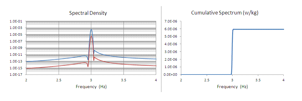
Figure 9. Same as Fig. 8 but with the drive frequency changed from 1 Hz to 3 Hz. The maximum drive acceleration magnitudes (at the peak of the Gaussian) were the same for the two cases; i.e., 0.02 m / s2.
The total power for Fig. (9) is 6 × 10⁻⁶ w/kg to two significant figures. Three times this number is greater than the total of Fig. 8 by 7 or 8 percent. An inspection of the line shape of Fig. 9 reveals that the difference from zero is the result of numerical integration errors. It could be reduced by using a larger number of FFT points than 1024 and reducing the 0.1 s step size. Such was deemed
unnecessary for present purposes.
Case 3 - a drive combination of 1 Hz and 3 Hz
Since the oscillator is linear, a drive which contains both signals should yield a total power that is just the sum
of the two totals mentioned;
i.e,. 1.7 × 10⁻⁵ w/kg + 6.0 × 10⁻⁶ w/kg = 2.3 × 10⁻⁵ w/kg
So a third case was simulated, as shown in Fig. 10.
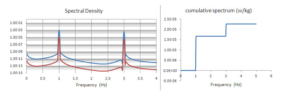
Figure 10. Result of drive involving both 1 Hz and 3 Hz accelerations. The total power (peak of the csp graph) corresponds
to 2.3 × 10⁻⁵ w/kg as required for consistency with Parseval's theorem.
Transfer Function Influence
For all of the above external drive cases, the drive frequency was higher than the oscillator's natural frequency. For these cases the
acceleration of the mass was virtually equal to the acceleration of the drive. Because the simulation calculated the psd using mass
acceleration, there was therefore no correction involving the system's transfer function.
For a drive
frequency less than 0.355 Hz, a transfer function correction would have been necessary. The theory for such corrections assumes steady state motion and the correction is different depending on whether the calculation of the psd works with mass motion based on the acceleration response or the displacement response. This difference is shown in Fig. 11.
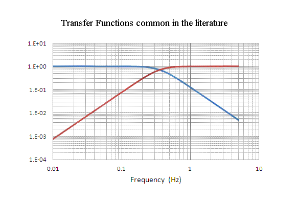
Figure 11. Illustration of transfer function differences that must be considered when calculationg the psd.
These curves represent mass displacement response to ground acceleration drive (blue) and ground displacement drive (red).
It is important to understand some transfer function subtleties. Neither of the graphs of Fig. 11 (derived in ref. 2) applies
directly to the simulations of this study. Ground displacement was never utilized in the calculations, because of integration errors that would derive
from integrating twice the (more) fundamental (specified) ground acceleration drive. Most important for these simulations is a
transfer function corresponding to mass acceleration in response to ground acceleration. It is equivalent to the red curve of Fig. 11, since for steady state motion below the corner frequency, the ratio of ground acceleration to mass displacement is wo2. This relationship was found to be true for the simulations, and the same is also true for
a `simple' gravitational pendulum [3].
A drive at 0.1 Hz was simulated with the same peak acceleration of 0.02 m/s2 of the earlier cases and agreement between theory and experiment proved worse for an obvious reason. As was noted, the well known expressions for the transfer functions used to generate Fig. 11 are based on the assumption of steady state motion. With every simulation involving a given drive frequency whose level is significantly above noise there are significant transients. Because a theoretical correction for these transients is virtually intractable for present purposes, we see yet another example for seeking to maximize a seismometer's bandpass.
Another important consideration is the type of sensor used to monitor the motion of the mass. Unlike the present simulations
in which the FFT was computed using mass accelerations; in a seismometer the ground acceleration can be estimated directly from a sensor that measures mass displacement. For drive frequencies below the corner frequency of the instrument, no transfer function correction is required. We see then an advantage to working at low frequencies with such a displacement sensor, so that no substantial correction for instrument response is needed. With a velocity sensor, frequency dependence of the necessary correction will introduce errors because of transients.
Case 4 - Simulation of oscillator response to noise
The simulation that was used to produce the graphs in Fig. 2 is now discussed.
The drive acceleration record was generated with the Excel random number generator using a normal distribution with a mean of zero and a standard deviation of 1 × 10⁻⁵. A graph of the record is shown in Fig. 12, along with a plot of the velocity, which was used
to calculate the work done against friction-so that a comparison could be made with the psd-calculated total power. It is worth noting
that the velocity distribution is the same as Brownian noise, since it was obtained by integrating over the acceleration.
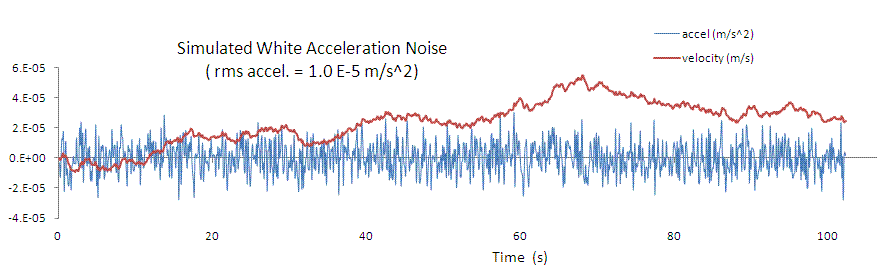
Figure 12. Low level acceleration record used to simulate the oscillator's response to white noise.
To avoid the difficulties previously mentioned, associated with transfer function correction, the corner frequency of the oscillator was for this case lowered to 0.005 Hz, below the lowest frequency of mass motion. For a Q of 0.707 in this case
b = 0.02236. The psd was then calculated as in earlier cases, and the results are displayed in several forms shown above in Fig. 2.
To explicitly illustrate the pink character of the power spectral density for this noise, Fig. 13 is provided.
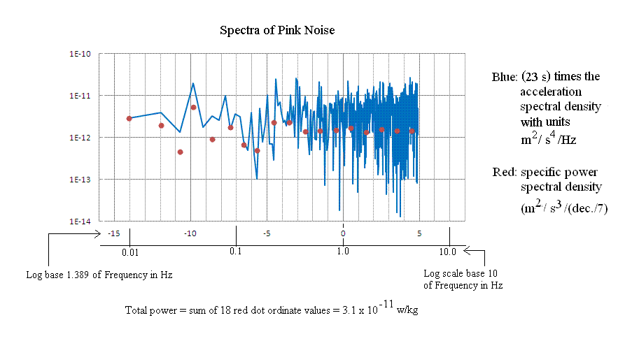
Figure 13. Specific power spectral density of pink noise illustrating the natural units of w/kg/(one-seventh-decade)
The blue spectrum corresponds to working`blindly' with the asd and plotting it in log-log form. Multiplying the asd by the scale factor of 23 s = 1/(2 p Q flowest) causes it to agree with the psd. This scale factor difference between the psd and the asd is due to the `compression' feature of the FFT when using the logarithm. As frequency increases, the number of points per d[log(f)] increases because the differential equals df/f, and df = constant. The only way to properly account for this compression, as when doing an integral to get the total power, is to multiply the psd in w/kg/FFT pt. by f/flowest before plotting in log-log form. The multiplicative f term causes it to become the same (apart from a scaling factor) as the asd plotted log-log but ignoring the influence of the transformation to log coordinates.
Comparison of the powers
Noted in Fig. 13 is a number for the total power obtained by summing the eighteen bin values denoted by the red dots. The same value of
3.1 × 10⁻¹¹ /w/kg was obtained by integrating over the full frequency range of psd(f)df where the units of psd are w/kg/Hz.
The average power using Eq.(6) for the work done against the damping force yielded the value 3.3 × 10⁻¹¹ /w/kg.
Their difference of 6% is consistent with numerical errors in the discrete integrations performed, for the step size of dt = 0.1 s. Therefore this case is seen to also be consistent with Parseval's theorem.
Conclusion
A host of different cases have been here simulated numerically. They demonstrate mutual agreement with respect to (specific) power spectral density calculations performed, and in every case the calculated psd is consistent with Parseval's theorem. Therefore it can be confidently concluded that the natural (true) set of units for psd are either w/kg/Hz = m2/s3/Hz for linear plots or w/kg/(user specified decade or octave) for log plots.
Bibliography
1. Hysteretic damping is treated in ``Damping Theory'' by R. Peters, in Vibration Damping, Control, and Design, ed. C. V. de Silva,
CRC Press (2007).
2. Transfer functions are treated by Erhard Wielandt in ``Seismic Sensors and their Calibration'', a chapter from the ``new Manual
of Observatory Practice, ed. P. Bormann & E. Bergmann, online at
http://www.geophys.uni-stuttgart.de/oldwww/seismometry/man_html/index.html
3. R. Peters, ``Tutorial on gravitation pendulum theory applied to seismic sensing of translation and rotation'', in BSSA
Special Issue on Rotational Seismology'' (2009).
File translated from TEX by TTH, version 1.95.
On 2 Jan 2012, 22:35.