Abstract

As a tool for the analysis of dynamical systems, the classical phase space portrait first used by Willard Gibbs is widely employed. The autocorrelation of a time signal is also well known. Our article describes a synergetic exploitation of the pair, in which properties of the autocorrelation are used to advantage for the study of quasiperiodic time domain signals.

Background

We have been attempting to assess the viability of seismocardiographic (SCG) records for the diagnosis of heart abnormalities. A variety of the many known human body complexities have made our task challenging. Among the various analytic methods we have considered are some of the now-common tools for the treatment of chaotic systems, starting first with mechanical systems, but more recently applied to studies of the human heart [2]. Although some of these methods looked initially attractive, they have proven less than satisfactory. Living systems do not adhere to the `deterministic' basis of chaos theory. In other words, it appears there will never be a well-defined, reasonably simple, non-linear differential equation to describe the mechanics of a living heart.

Among other complications, a beating heart is significantly influenced by its environment. For example, in general there are measurable differences between male and female subjects that derive from differences in the size and shape of the chest. An ideal SCG `sensor' would be one that could match the performance capabilities of the human ear-such as immediately being able to distinguish between a piano and a violin playing the same note.

What makes the `timbre' of a heart generated signal especially difficult to classify is its quasi-periodicity, meaning that the `drive' is not essentially monochromatic, as with the classic systems of chaotic type. This makes the phase space trajectories even more `cluttered than usual'; and Poincare `sectioning' to reveal precise values of fractal geometry is not straightforward, if even possible.

Phase Space Trajectory

One convenient property of the phase space trajectory is the manner in which dynamical features of a system are revealed naturally in a bounded space. Two illustrative cases are provided in Fig. 1.

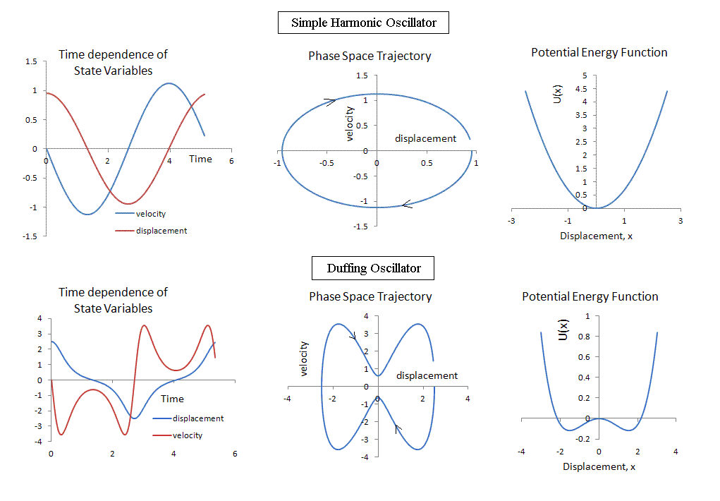
Figure 1. Examples of phase space differences between the undamped, undriven simple harmonic oscillator (top middle plot) and the undamped, undriven Duffing oscillator (bottom middle plot). The left-side time plots show in each case only one nearly complete cycle of the monochromatic signal for which there are no transients.

These phase space trajectories were generated by plotting velocity (the time derivative of displacement) on the vertical axis versus the displacement on the horizontal axis. In classical mechanics it is usually the momentum that gets plotted (a 'conjugate' quantity that is the derivative of a generalized coordinate and which in the simplest case is the product of mass and velocity). The equation of motion relating the pair as a function of time is elegantly solved by means of Hamilton's canonical equations. For a given case the state variables with which Fig. 1 was generated were obtained by numerically integrating a 2nd order differential equation of motion. The potential energy function U(x), that is also shown, allows one to specify the force acting on the mass. The net force is given by the negative derivative of U with respect to the displacement x. This force is in turn used with Newton's 2nd law to obtain the eqution of motion. For reason of processor errors it is better in numerical calculations to work with two coupled first order equations rather than to integrate the 2nd order equation twice.

Autocorrelation

For a sampled (digital) record of measurements the autocorrelation is defined by

where N is the total number of measurements, k varies between 1 and N, and Y_i, ( i = 1, 2, ..., max of N ) are the measured values for which their mean value is <Y>.

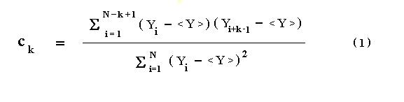
An example of the use of Eq.(1) to calculate an autocorrelation is provided in Fig. 2.

Figure 2. Autocorrelation (lower graph) calculated from a two-cycle square wave of finite duration (upper graph) using Eq. (1). In contrast to the 256 points that were used to simulate the square wave, only every fourth point of the autocorrelation's full set were calculated for the plot that is shown. Had all 256 values been computed, a near continuous 'decaying sawtooth wave' would have resulted.

Rather than use the cumbersome Eq. (1), the autocorrelation is more easily and quickly calculated by means of the fast Fourier transform (FFT), by taking advantages of the Wiener Khinchin theorem. As noted elsewhere [1], care must be taken with the use of this method to account for the influence of causality (influence of the finite duration of the signal treated).

Fig. 3 shows (left graph) that a proper use of the FFT to calculate the autocorrelation (blue curve) gives the same result as Eq. (1) (now red dots that were the blue dots of Fig. 2). Also shown on the right is the result of calculating the (cyclic) autocorrelation that does not agree with Eq.(1). Details concerning these calculations are provided in reference [1].

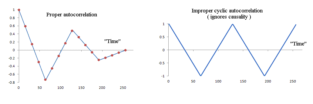
Figure 3. Demonstration (left) of the equivalence of Eq.(1) and the use of the FFT with the Wiener Khinchin theorem to calculate the "proper" autocorrelation. The cyclic calculation that gave the right graph does not agree with the defining relationship for the autocorrelation.

One attractive property of the autocorrelation as a basis for trajectory portraits, involves its secular decrease with time t. For a record whose total duration is T, the autocorrelation takes on the value of unity at t = 0 and decreases to zero at t = T. This property is illustrated for the classical oscillators of Fig. 1 by the plots of Figure 4.

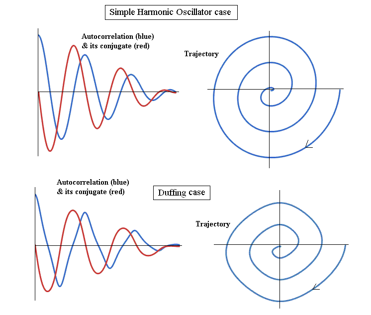
Figure 4. Autocorrelations (left) and trajectories generated using them (right) for the oscillators of Fig. 1. These trajectories (later referred to as portraits) were generated by means of the 'integral' form that is discussed below.

Conjugate Variable Choice

The classical phase space trajectory uses the time 'derivative' of the waveform of a'signal' as the 'conjugate' with which its portrait is generated. A useful alternative conjugate is the 'integral' of the 'signal'. Illustrations of both portrait types are provided in Fig. 5, where the so-called 'signal' in the top half of the figure is the autocorrelation represented by the lower graph of Fig. 2.

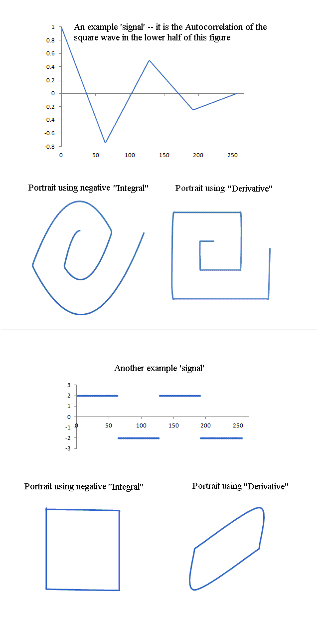
Figure 5. Illustration of various portrait characteristics for different combinations of 'signal'-plus-conjugate.

It should be noted that the 'derivative' and 'integral' with which the portraits are generated is in each case a coarse approximation of numerical processing type. It is computed as follows. Let the column vector representing the 'signal' be designated by s_i where i = 1, 2, ..., N. In figures 2, 4 and 5 above, N = 256. The choice of 256 = 2⁸ is consistent with the constraint required of a 'proper'set (as an integer power of 2) for calculations of the Fast Fourier Transform [3]. Two different phase portraits of the type being presently discussed are possible. The 'derivative' of s is the column vector d_i that is initialized by d₁  =  0 and for i > 1 is given by d_i  =  s_i+1 - s_i. For example, such was used to generate the lowest right portrait of Fig. 5. It was plotted with the default settings in Excel, whereby it is unnecessary that the user be concerned with particulars of scale factors. The same auto-scaling is available when the portraits are generated by means of Mathematica.

Influence of Noise

The influence of signal noise on the portrait is significantly reduced by working with the negative integral of the signal as the conjugate with which the portrait is generated. The negative rather than positive integral is chosen so as to yield for the portrait the same direction of circulation as with the derivative case, Thus if we initialize its column vector with a zero as before, then for i > 1 the negative 'integral' is calculated using I_i+1  =  I_i - s_i+1. As compared to the derivative form, The integral form is dramatically impervious to random noise present with the signal, as demonstrated by comparison of the pair of lower portraits of Fig. 6.

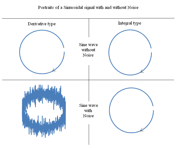
Figure 6. Simulated portraits showing the large influence of random noise on the derivative form of a phase portrait. The rms noise level was for both cases the same tenth of one percent of the sine amplitude.

Influence of Variable Drive Period

The autocorrelation phase portrait is especially useful for the analysis of signals having a variable rate. An example is provided in Fig. 7, which has similarities to the structure of the r-wave components of the electrocardiogram of a healthy subject.

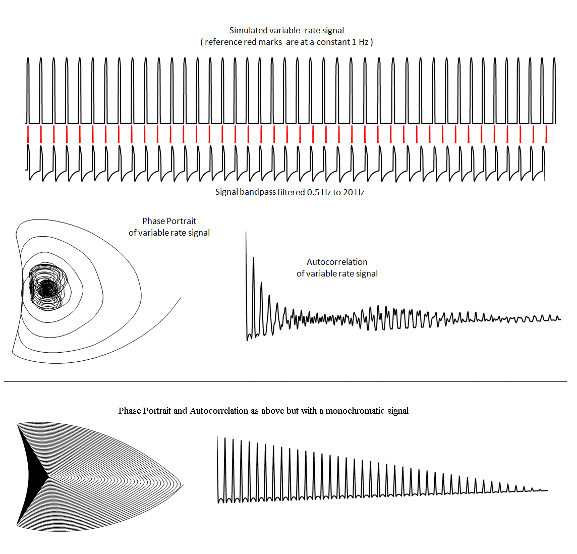
Figure 7. Simulation example of the influence (top) of variable rate on the phase portrait of a signal with varying period between pulses. For comparison, the fixed-period (monochromatic) corresponding case is also shown (bottom).

EKG case

The influence on phase portraits of variable rate of the normal heartbeat is illustrated in Fig. 8.

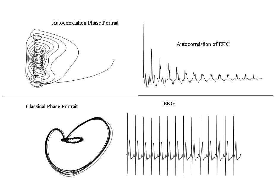
Figure 8. Comparison of the autocorrelation phase portrait (top) with the classical phase space trajectory (bottom).

Rate variability is revealed in the upper phase portrait through localized trace 'darkening' because of influence (in general) from the presenceof minima/maxima in the decay of the autocorrelation. By contrast the same variability is not readily obvious in the lower classical trajectory.

Conclusions

The novel tool described in this article, called the autocorrelaton phase portrait, derives from the physics concept called Phase Space. The conventional phase space trajectory is generated from the state variables of displacement and velocity (derivative of displacement). A portrait generated by the present method is a two-dimensional graphical figure with some similarity to those of classical type. It does not, however, derive directly from the displacement, but rather from the autocorrelation of the displacement. It has a resulting secular decline toward a 'zero' (or center) point. With some systems of complexity type, this feature allows a greater visual insight into dynamical properties of the system that are 'mapped' thereby.

Acknowledgment

This work was supported by the National Institutes of Health Grant titled ``Three dimensional cardiac accelerometry for low-cost, non-invasive cardiac monitoring'', awarded 06/14/2010.

References

[1] R. D. Peters, ``Autocorrelation and Causality (subtleties of the FFT)'', online at http://physics.mercer.edu/hpage/autocorrelation/subtlety.pdf

[2] Gari D. Clifford, ``ECG Statistics, Noise, Artifacts and Missing Data'', Ch. 3 of Advanced Methods and Tools for ECG Data Analysis, Editors G. Clifford, F. Azuaje, & P. McSharry, Engineering in Medicine & Biology Series (2006).

[3] R. Peters, ``Graphical explanation for the speed of the Fast Fourier Transform'', online at arxiv.org/html/math.HO/0302212