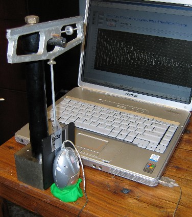
Figure 1. First pendulum that was tested. The mouse is held in place with play-doh.
Motivation
Throughout its long history, the pendulum has been one of the
most important tools of science education. It is true that
visual-only observations of a swinging
pendulum provide a measure of conceptual understanding.
But a true appreciation
for the physics of just a single configuration of
this instrument that
exists in a variety of useful forms-
requires an extensive study of quantitative type. Such
quantitative studies
are impossible without some reasonably accurate
(and hopefully easy) means for
measuring the displacement of the pendulum.
Previous Sensor Types
The method we are describing has been used to study simple harmonic
oscillation of a mass on a spring [1]. What is missing from that
publication as compared to the present paper is the attention we give to
the software that allows for trivial implementation of a powerful, yet
user-friendly acquisition system. Additionally, we describe a novel,
low-friction axis for pendulums.
In yet another paper [2], the light source of the mouse has been replaced by a diode laser; although the CCD of the mouse is still used with a modified tracking algorithm. As compared to the present approach, this requires additional work that most teachers will not want to do.
Among older types of sensors, a variety of different technologieis have been used through the years to study mechanical oscillators in general. The most common (and successful) electronic devices have been ones that were either (i) optical, (ii) capacitive, or (iii) inductive type. One of the present authors (RDP) has in the span of two decades done many experiments with capacitive sensors, having patented the first fully-differential form.
Each of these previous electronic sensors requires an auxiliary analog to digital converter (ADC), which is typically an expensive addition. The cheapest commercial ADC known to the authors costs about $25. Unlike the mouse sensor being presently described, this package (like all others) is not specifically tailored to the study of pendulum types having the greatest interest of educators.
Benefits of the Mouse-Sensor/Software Package
There are two significant differences between the present method of
pendulum sensing and the methods used in the past.
(1) The software designed for the mouse sensor has been tailored for specific application to pendulum configurations of interest to science educators. Consequently, it is both powerful and user friendly. In the hardware arena, advantage is being taken of the successes that derive from enormous engineering efforts that went into the development of the computer mouse as we now know it.
(2) For those teachers who (i) already use an optical mouse with their computer, and (ii) have access to the internet, the cost of this sensor is essentially ZERO. The reason for zero-cost is that the executable software to operate the mouse is available for free download at http://faculty.mercer.edu/lee_sc/research/mousemotion/InstallMouseMotion.zip (Note: You need to send an email to Dr. Lee ( Lee_sc@mercer.edu ) to get a password required for extraction of the .zip file, since he ``would just love to know where this little program has found home''.)
Setup
Shown in Fig. 1 is a photograph of the first pendulum that was used to evaluate the methodology. The pendulum hardware derives from scavenged/reworked materials that were once part of an old pan-balance.
Figure 1. First pendulum that was tested. The mouse is held
in place with play-doh.
Physical contact is not permitted between the mouse and the surface onto which the light source is directed for monitoring. The mouse is able to detect the motion of that surface as long as the gap-space between the two is not greater than about 1 - 2 mm. In the picture of Fig. 1 this surface is a flat section of a floppy disk that was taped to the bottom end of the rod that is part of the compound pendulum. The axis of the pendulum is in the form of knife-edges resting on pieces of sapphire.
Lest the pendulum be adversely affected by friction of the axis, it is important that very hard materials be used to form the contacting surfaces that form the axis. One of the best and readily available means for providing such an axis is shown in Fig. 2.
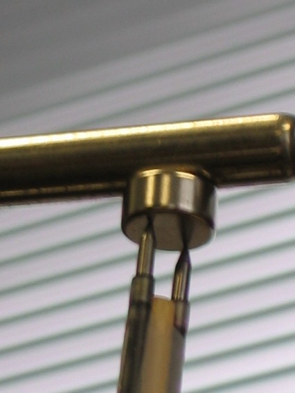
Figure 2. Axis comprising a pair of replacement ball-point-pen
inserts supporting the pendulum and hanging from a rare-earth magnet.
The pendulum whose top-only is pictured in Fig. 2 is 39 cm in length. The very hard, small tungsten-carbide spheres of the pen ends contact the magnet through the attractive force on the ferrous metal tubes that hold them. The force is great enough to support about 200 g total mass of pendulum for the 1/2 - in magnet here used. Faintly visible in the photo is a portion of the tape with which the pens were secured to the 1/8 - inch wooden dowel that connects the pens at the top. It should be noted that not every type of ball point pen can be used this way; however, many inexpensive, acceptable brands are commonly available, at least in the United States.
Instead of the floppy disk shown in fig. 1, a small piece of cardboard (approximately one-third the size of a business card, cut perpendicular to the small dimension) was butt-end attached to the bottom of the wooden rod. Thus the mouse could rest (more stably) in an orientation that is 'upside down' to the usual-for-computer-use orientation.
Example Data
Shown in Fig. 3 is an example Low-Q free-decay record of this wooden-rod pendulum. Data used to generate the plot with Excel were first saved and afterwards filtered to remove mean position variations that occur with characteristic times that are long compared to the period of the pendulum,
Figure 3. Example free-decay record generated with the optical
mouse sensor. The 'fit to the turning points' used to calculate the
quality factor of 32 is also shown.
In general there is a tendency for the mean position of the displayed waveform to migrate in spite of the absence of actual physical migration. This is thought to result from two factors: (i) difficulty of achieving a perfect fixed-gap parallelism of the mouse bottom surface and the near planar piece of the pendulum bottom that it watches (piece of business card), and (ii) an asymmetry in the treatment of the turning points of the motion built into the algorithm used by Windows in the computer. The bandpass filter that has been added to the software eliminates drift of the realtime display on the monitor, and reduces high frequency noises (including discretization errors due to the dpi size). What is saved to memory of the computer is not filtered, but we supply the filter in a separate package for those who wish to use it.
The initial amplitude of the pendulum was just over 100 counts, corresponding to approximately 12 mrad displacement. For the 39 cm long pendulum, the corresponding linear displacement of the bottom end of the rod was approximately 0.5 cm.
About the Quality Factor Q
Textbooks usually describe the approximately exponential decay of the turning points shown in Fig. 2 by means of a coefficient b having units 1/s. This coefficient should not be referred to as a damping `constant', since it depends in a complex manner on a variety of factors including air density as well as air viscosity [3]. The exponential curve of Fig. 2 corresponds to 113 exp(-0.08 s-1t), where b = 0.08/s. The alternative (present) means for specifying the decay is Q = p/(b T) where T is the period. The quality factor is defined in terms of the energy loss per cycle D E according to Q = - 2p E/DE.
A convenient (easy) way to roughly estimate the Q of an exponential decay is to count the number of cycles required for the amplitude to fall to 1/e = 0.37 of its initial value. Then multiply this number by 3.14 to get Q.
Shown in Fig. 4 is the spectrum calculated using the Excel FFT (Fourier analysis tool) operating on the Fig. 3 data. To use the Fourier Analysis program of Excel, one must employ the 'tool-pak' add-in. The motion of the pendulum at these small amplitudes is nearly isochronous, with a period of 1.22 s, which was estimated by taking the reciprocal of the peak value of Fig 4 (read off the Excel plot by 'highlighting' the graph and then placing the cursor at that point).
Figure 4. Fast Fourier Transform (FFT) Spectrum of the
the record shown in Fig. 3.
The considerable damping of the pendulum is due mainly to air viscosity. At the small amplitudes of the pendulum type used for this work, the damping can be adequately approximated, for most purposes, by assuming that the damping torque is proportional to the first power of the velocity. This is, however, a terrible approximation for many of the pendulums studied by one of the authors (RP). The reader who would like extensive information about nonlinear damping (not just from quadratic-in-the-velocity air influence, but also from hysteretic damping from internal friction of structures) is referred to reference [4].
High-Q Free Decay case
A simple means to increase the Q of the wooden rod pendulum is to add some mass to it. For the next decay case, this was accomplished by placing a small steel roller ball bearing around the rod at its bottom (a `bob' mass of about 30 g, resting on the cardboard piece attached with scotch tape to the bottom of the rod).
After manually intitializing the motion (pushing with a finger on the bearing and then releasing), the data for the decay of Fig. 5 was generated. As before, post-filtering was employed and the text file of the output from the filter was copied into Excel. The free-decay plot was then generated, along with the exponential fit as before.
Figure 5. Example free-decay record produced in the same manner as
Fig. 3, except after modifying the pendulum by adding some 'bob' mass.
Also in analogous manner to the spectrum of Fig. 4, the FFT of the data of Fig. 5 was used to produce Fig. 6.
Figure 6. FFT Spectrum of the record shown in Fig.5. The half-width
of the pendulum's fundamental spectral line is less than that
of Fig. 4, consistent with the higher Q (in accord
with the uncertainty principle).
Because the pendulum is of 'physical' rather than 'simple' type, the period of its oscillation was almost unchanged by adding the bob mass at the bottom of the rod. The increase in its moment of inertia by this means, without causing a significant change in the damping, allowed for a readily-achieved five-fold increase in the quality factor.
Closing comment
This pair of differing-Q, free-decay cases, studied by means of a user friendly but powerful means for collecting and analyzing a pendulum's motion-represents in the minds of the authors a significant new pedagogical tool for the study of mechanics.
Acknowledgement
Someone who largely influenced the authors to sense pendulum
(seismometer) motion by the means described in this paper
is Denny Goodwin of Demopolis, Alabama. The authors gratefully acknowledge
Rev. Goodwin's contributions to both this effort and also to another sensor
project (having much greater resolution) that uses the AD698 integrated
circuit sold by Analog Devices.
Bibliography
[1] T. W. Ng & K. T. Ang, "The optical mouse for harmonic oscillator
experimentation", Am. J. Phys., vol. 73, No. 8, (2005).
[2] D. Jiang, J. Xiao, H. Li & Q. Dai, "New approaches to data acquisitions
in a torsion pendulum experiment", Eur. J. Phys. 28, 977-982 (2007).
[3] R. Peters, "Nonlinear damping of the linear pendulum",
http://arxiv.org/ftp/physics/papers/0306/0306081.pdf
[4] R. Peters, "Damping theory", ch. 2 of Vibration Damping, Control,
and Design, ed. C. de Silva, CRC Press, ISBN 1420053213 (2007).