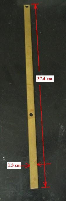
Figure 2. Photograph of the dismounted Kater pendulum, showing the holes which provide means for axis rotation.
Theory of the classical driven, damped, simple harmonic oscillator is basic to the training of students in physics and engineering. Unfortunately, improvements in understanding of some of the lesser known motions predicted by theory have suffered because of difficulties in their experimental demonstration. Recently developed commercial products, of both hardware and software type, now allow for extensive comparisons of theory and experiment for this foundational dynamical system. The significant increase in experimental capability results because three essential components are finally able to function synergetically. These are: (i) an adequate sensor, (ii) a powerful interface to a personal computer, and (iii) powerful yet user-friendly software with which to analyze the records created by (i) and (ii).
The recent trend of commercial analog to digital converters (adc's) is mainly toward `plug-and-play' connection to the USB port of personal computers. These serial devices suffer from significantly restricted maximum sample collection rates as compared to earlier parallel port devices. Additionally, the resolution of inexpensive serial units has been poor-only 12 bit converters for adc's in the $100 price range. Using two's complement (one bit for algebraic sign), and typically having no range selectability (hardwired at plus and minus 10 volts), these converters cannot resolve voltage variations smaller than 5 mV.
By contrast, recently developed inexpensive 24-bit parallel-port adc's can resolve signal variations more than three orders of magnitude smaller (below 3 mV). (For the present work, Symmetric Research's PAR1CH [1] was used, which sells for $150). As compared to the USB-devices, the greatest deficiency of this instrument (and other similar ones) remains that of software support. Fortunately, as will be shortly illustrated, the binary-stored records they generate can be easily transformed into ascii form, using code written in QuickBasic (or VisualBasic). Once transformed, these records are easily studied with the user-friendly but powerful (and free) waveform-browser software that is available from Dataq, Inc [2].
Sensor: A number of operationally different sensors might possibly be used for studies of the present type; but historically, the requirements of the sensor have not been achieved with ease in very many cases. The measurement of oscillator position must be precise over a large dynamic range, and the sensor must possess outstanding linearity. A position detector that inexpensively meets all these requirements, and which was used for the present experiments, is the fully-differential capacitive sensor patented by the author [3].
Software: The present author has written his own dos-based code for many experimental studies of the past. Especially important to the various algorithms routinely employed has been means for displaying features of the frequency domain. The fast Fourier transform (FFT) has become the mainstay for these calculations. Its greatest versatility is realized when one can work with readily selectable time windows, subject to the constraint that the total number of sample-points N is expressible as N = 2n where n is an integer. Such versatility is critical to the exploration of an archived record for features that would not otherwise be readily noticed. Means for discovering time-evolutionary properties of a dynamical system are especially improved when one is able to easily compress records by means of input averaging.
As the reader may appreciate, generation of code to accomplish all the things just indicated is a daunting task. The waveform browser indicated in reference 2 is a windows-based software package that successfully met the challenge. Although a great deal of engineering development must have gone into its creation, it is nevertheless free! No doubt this will serve to increase Dataq's hardware sales; as evidenced by the fact that the present author was thusly motivated to purchase three of their DI-700 adc's (no longer marketed, being replaced by their model DI-710).
The pendulum was designed by the present author [4] and is
sold by Tel-Atomic Inc (``Student-friendly Kater precision pendulum'',
described at the company webpage http://telatomic.com).
A picture of the dismounted pendulum is provided in Fig. 2.
Figure 2. Photograph of the dismounted Kater pendulum, showing
the holes which provide means for axis rotation.
When used to estimate the Earth's field g � 9.8 m/s2, the pendulum is swung about first one and then the other axis formed by mounting the instrument on a `knife' edge passing through a hole in the brass rod. For the present experiment, only oscillation using the end hole was employed. For either hole, the nominal frequency of the instrument is 1 Hz. The `knife' edge used for the present experiment is provided by the shaft of the screwdriver located in the upper clamp. It was oriented to provide a pivot from `face-pairs' that intersect at 90 degrees. (one of the edges resulting from the four-fold rotational symmetric shaft connecting handle and flattened usual working end).
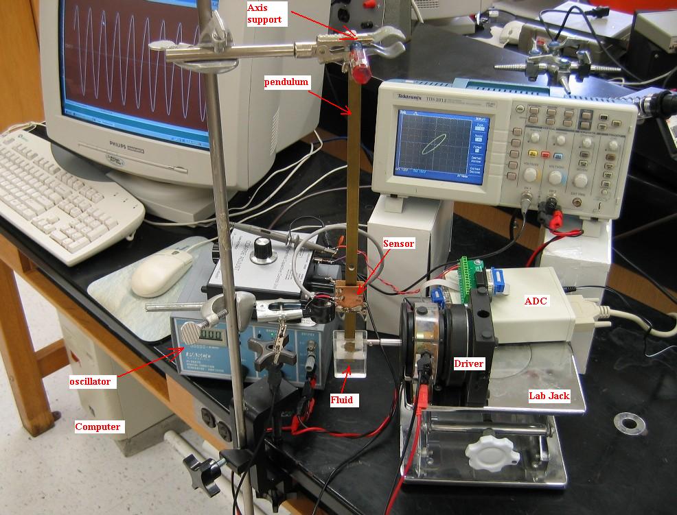
Drive: The pendulum is excited into motion by means of the fluid in the clear plastic container attached to the driver. This driver (mechanical vibrator SF 9324) and the associated oscillator (Digital function generator-amplifier PI 9587C) with which it is energized, are both sold by Pasco.
Sensor: A closeup photograph of the sensor is
provided in Fig. 3.
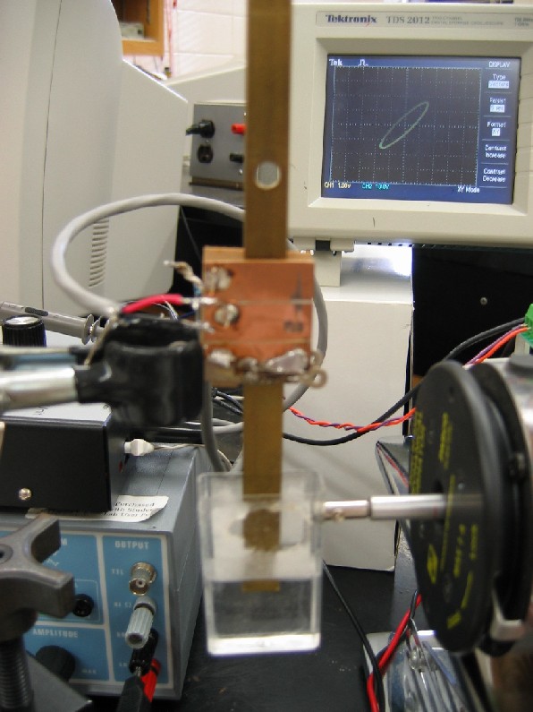
Figure 3. The area-varying SDC capacitive sensor
used to measure pendulum position.
The plates were in this case formed by filing away copper (along straight lines) from printed circuit board material, to form various of its insulator strips. The electronics to operate the sensor was for the present work the unlabeled box that is more fully visible in Fig. 1 (unit with the black zeroing knob on the top). It is no longer sold by Tel-Atomic, but plans are underway to market an inexpensive general purpose autozeroing package that works with the sensor plates in the manner illustrated by the sensor tutorial that is online at http://physics.mercer.edu/petepag/tutorial.html.
Other Equipment: Visible in the background of Fig. 3 is an oscilloscope xy trace in which drive voltage is supplied to the y-axis and sensor output voltage to the x-axis. The oscilloscope chosen (Tektronix model TDS 2012, used in Mercer University Physics general education laboratories) is of digital rather than analog type, since it is difficult to meaningfully display slowly varying waveforms on an analog instrument. The oscilloscope is ideal for viewing the pendulum's motion in real time, and provides the simplest means for generating a resonance curves, whether it be frequency dependence of amplitude or of phase difference of pendulum relative to drive.
| (1) |
where the force Fv derives from the viscosity of the fluid and is several times more influential than the fluid's inertial contributor Fi. The natural (eigenfrequency) of the oscillator is w0, and the quality factor Q is defined as 2p times the ratio of the energy of oscillation to the energy loss per cycle. The two forces are modeled as follows:
| (2) |
| (3) |
To solve for the steady state motion of the oscillator, one substitutes equations (2) and (3) into (1) to yield
| (4) |
Assuming the entrained oscillator response to be x = A ei wt one obtains
| (5) |
The resonance features inherent within the expressions of Eq(6) are
illustrated in Figures 4 and 5.
Figure 4. Bode plot for the amplitude response of the oscillator
for two different values of Q. The red curves correspond to c = 0.
Figure 5. Phase of oscillator relative to drive for two different
values of Q. The red curves correspond to c = 0.
Amplitudes of oscillation approach noise levels for |Log(f)| > 0.2.
Thus the difference between the c = 0 and c = 0.25 cases is
inconsequential to the amplitude response. The same is not true of
the phase, however, as illustrated in Fig. 6.
Figure 6. Shift of oscillator phase (c = 0.25, black curve) as compared
to the c = 0 case (red curve). For this case Q = 7.2.
Notice that the oscillator leads the drive by p/2 for drive frequencies
well below resonance, whereas it lags the drive by p/2 for
frequencies well above resonance. This is in contrast to the usual
textbook case of transition from in-phase (below) to lag by p (above).
The usual case is accommodated by the present theory by letting c become
much larger than 1, as illustrated in Fig. 7.
Figure 7. Comparison of oscillator phase for c = 0.25 (red)
and c = 20 (black).
Differences between the line of theory and the points of the data are too small to be visible; however, quality of the fit can be assessed from the residuals, which have been plotted as five times the difference. The equation used for this Excel plot was 0.164 exp(-.058 t) cos (2p · 1.00 t - 0.740), where the time step was D t = 0.01 s (corresponding to the 100 samples/s data-collection rate of the PAR1CH). Of the parameters indicated in this expression, both the 0.058 and the 1.00 were obtained directly from FFT computations using the Dataq waveform browser operating on the ascii-transformed data. A single calculation is adequate for determining the frequency to about 2% (precision governed by the Nyquist frequency, itself determined by the sample rate and the total time of data collection). A series of four FFT computations separated in time by Dt = 10.7 s yielded Q from the trendline whose slope is indicated in the lower graph. The other two parameters were obtained by trial and error using Excel's autofill function. It is a simple matter to make a parameter change, autofill upward, and watch the resulting change to the graph of the residuals. Fewer than a dozen quickly administered trial and error variations in this manner is typically required to essentially minimize the residuals, which are never zero because of oscillator noises involving both amplitude and phase. Other, more sophisticated methods could undoubtedly be employed to provide such a multi-parameter ``best'' fit but the one just described has proven to be very satisfactory.
It should be noted that exponential decay does not guarantee that the damping mechanism of an oscillator is linear. Nonlinear hysteretic damping, due to internal friction as an example, causes an exponential decay even though the equation of motion does not obey Eq.(1) with the right-hand-side set to zero [5].
The use of the short time Fourier transform is a powerful, yet user-friendly means for accurately estimating the Q of an oscillator. The free-decay method employed is described on page of 21-25 of reference 5. The equation for Q in the lower graph of Fig. 8 corresponds to Eq.(21.4) of that reference.
The second harmonic of pendulum motion is the only visible one when operating at large amplitudes. It is barely visible as a notch at 40 dB below the fundamental; i.e., one hundred times smaller in amplitude. The lower graph provides an estimate of system noises, which are expected to derive mainly from two sources: (i) electronics and (ii) turbulent eddies in the driving fluid. For the case shown (and all others of this article), the fluid used was mineral oil. When replaced with a rheoscopic fluid the eddies could be directly observed visually.
For the cases considered, because the sensor is linear within the operating range (amplitudes less than 20 mrad); there is no need for it to be accurately calibrated. If such a calibration were required, this could be accomplished by the optical lever technique; i.e., reflecting a laser beam from a mirror attached to the pendulum for given (known) deflections. A rough estimate of the calibration constant yielded the value 300 V/rad, which is small (because of the large gap spacing between stationary plates at 0.6 cm) as compared to some other sensor configurations. For example, a pendulum used by the author to monitor local diurnal accelerations over the last year operates (by means of an array form of the SDC sensor) at 5800 V/rad.
The more shallow the depth of pendulum-end placement, the larger is the Q and the smaller is the coupling force. In turn, one must wait longer for the motion to reach a steady condition. Shown in Fig. 10 is a shallow-depth case. It should be noted that the free-decay data of Fig. 8 was obtained with the pendulum oscillating at a slightly shallower depth in the fluid (yielding Q = 54).
The solid line fit to the data points (both amplitude and phase graphs)
were generated using Eq.(6).
The experimental measurements were
performed with the digital oscilloscope operating in the xy mode.
The phase was measured from dimensions of the steady-state ellipse
as indicated in Fig. 11.
Figure 10. High Q resonance response of the pendulum. The bottom
of the pendulum was 0.7 cm below the surface of the mineral oil.
The amplitude response has been plotted in relative (dB) units normalized
to unity, yielding 0 dB at the resonance peak.
Figure 11. Illustration of the method for estimating the phase
of the pendulum relative to the drive. Circulation around the
ellipse displayed on the oscilloscope
is clockwise above resonance and counterclockwise below resonance.
Shown in Fig. 12 is a case with the bottom end of the
pendulum operating at a greater depth in the liquid.
Figure 12. Low Q resonance response of the pendulum. The bottom of
the pendulum was 2. cm below the surface of the mineral oil.
In the Fig. 11 graph the resonance frequency appears to be slightly higher at 1.005 Hz than the free-decay eigenfrequency estimated at 1.000 Hz. At 0.5 % the difference is too close to experimental uncertainty to warrant discussion.
Figure 13. Illustration of the transient response that occurs
until the pendulum entrains with the drive (upper curve), when driven
at frequencies other than resonance (bottom curve).
For the non-resonance case, a beat is observed with a period of 10 s, which corresponds to the difference between the pendulum's natural frequency of 1 Hz, and the drive frequency of 0.9 Hz. It is interesting to observe (i) the initially large beat amplitude that is visible in the graph, and (ii) on the oscilloscope operating in the xy mode- the significant variations in phase that occur until the pendulum finally entrains with the drive.